Matrix Effect Analysis

Overview

This article explores how to evaluate the matrix effect in pharmaceutical analysis using a simple linear model.

👉 Try the open and free R version online: VALIDR MATRIX app

Objective

The goal is to assess the influence of the pharmaceutical matrix on the analytical signal across different analyte concentrations.
The comparison is made between samples prepared in the analytical solvent and those prepared from a pharmaceutical form containing the analyte in the pharmaceutical matrix (e.g. excipients), at identical known concentrations.

Demonstrating a matrix effect means that calibration standards should be prepared in the pharmaceutical matrix rather than in the solvent, to ensure accuracy.

The fundamental principle of the calibration is to establish a relationship between the analytical signal and the concentration of the analyte. A calibrant of known concentration establishes the signal–concentration relationship, which can be mathematically expressed as:

\[ \text{signal} = f(\text{concentration}) \tag{1}\]

That allows the analyst to back-compute concentration from a known signal:

\[ \text{concentration} = f^{-1}(\text{signal}) \tag{2}\]

if and only if the relationship Equation 1 is identical for calibrants and matrix samples, ensuring that the calibration curve remains valid across different matrix conditions. This requires that the analytical response is not influenced by the matrix composition, as any deviation would necessitate matrix-matched calibration standards.

For simplicity in this demonstration, we assume a linear response model (e.g. Beer–Lambert law for UV spectroscopy: ( A = ε·l·c )). Note that this should not be confused with the linearity of the method, as a linear response model does not guarantee method linearity systematically.

Modelling the Matrix Effect

We could postulate that the overall equation modelling the signal response can be written as a function of concentration and matrix: \[ \text{Signal} = f(\text{Concentration}, \text{Matrix}) \]{eq-3}

For a linear model, this can be expressed as:

y = β₀ + β₁·x + β₂·M + β₃·(x:M) + ε

Where:

• x = concentration
  
• M = matrix condition (0 = solvent, 1 = pharmaceutical matrix)
  
• β₂ indicates a shift in intercept
  
• β₃ indicates a change in the slope

If there is no significant matrix effect, then β₂ = 0 and β₃ = 0 and the model simplifies to: \[ y = β₀ + β₁·x + ε \tag{3}\]

If there is a matrix effect, the model with the matrix (M=1) can be expressed as: \[ y = (β₀ + β₂) + (β₁ + β₃)·x + ε \tag{4}\]

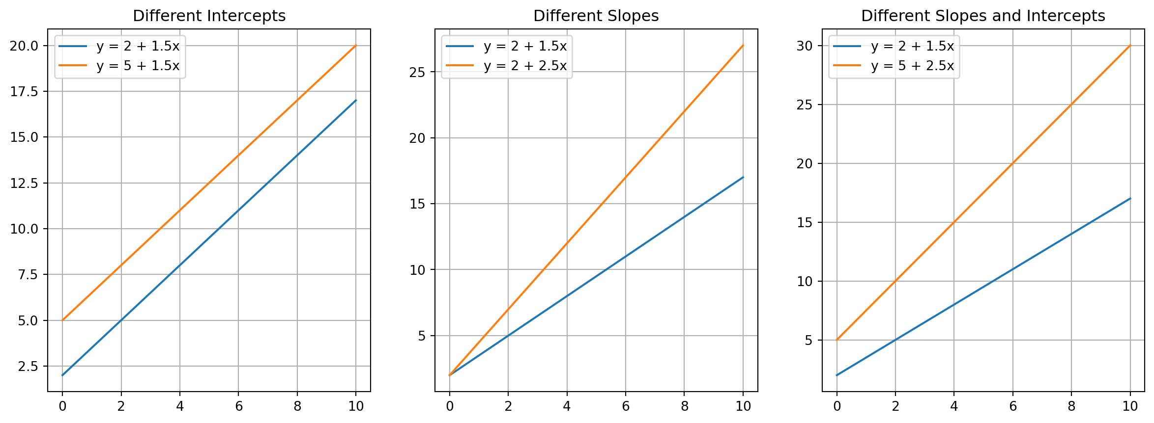
Statistically, to detect a matrix effect, we should perform a linear regression and test the significance of both the interaction term (β₃) and the intercept shift (β₂). This comprehensive approach ensures we fully evaluate the potential impact of the matrix on both the slope and intercept of the calibration curve.

Figure 1: Graphical representation of matrix effects: (left) different intercepts, (middle) different slopes, (right) different slopes and intercepts

Implementation in Python

We assume that a working Python environment with the required libraries are installed.

import pandas as pd #needed to load the data
import statsmodels.formula.api as smf #the linear regression model with formula syntax

# Load data
df = pd.read_csv('data.csv', sep=';', decimal=',') # adjust sep and decimal accordingly

# Model with interaction
model = smf.ols('SIGNAL ~ CONC * MATRIX', data=df) 

results = model.fit() 

print(results.summary())

Equivalent explicit form of the model:

model = smf.ols('SIGNAL ~ CONC + MATRIX + CONC:MATRIX', data=df)

Example dataset

The following folded code generates a synthetic dataset with 3 concentration points, 10 replicates each, and 2 MATRIXs (M=0 and M=1) for demonstration purposes.

import pandas as pd
import numpy as np
from sklearn.linear_model import LinearRegression

# Fix random seed for reproducibility
np.random.seed(42)

# Define concentration points (3 levels)
x_levels = np.array([1, 5, 9])

# Number of replicates per concentration level
n_replicates = 10

# Define linear functions with randomness
def line_with_noise(x, intercept, slope, noise_std=0.3):
    return intercept + slope * x + np.random.normal(0, noise_std, size=len(x))

# Generate data for M=0 and M=1 with replicates
x_all = []
y1_all = []
y2_all = []

for x_val in x_levels:
    x_all.extend([x_val] * n_replicates)
    y1_all.extend(line_with_noise(np.repeat(x_val, n_replicates), intercept=0, slope=1.5))
    y2_all.extend(line_with_noise(np.repeat(x_val, n_replicates), intercept=0.1, slope=1.2))

# Create a pandas DataFrame
df = pd.DataFrame({
    'CONC': np.concatenate([x_all, x_all]),
    'SIGNAL': np.concatenate([y1_all, y2_all]),
    'MATRIX': [0] * len(x_all) + [1] * len(x_all)
})

# Display the first few rows of the DataFrame
# print("DataFrame generated:")
# display(df.head(10))

# Save the DataFrame to a CSV file (optional)
# df.to_csv('matrix_data.csv', index=False)
# print("\nData saved to 'matrix_data.csv'.")

Example Output

In this example we’re reusing the dfgenerated above but you could load a csv data file using pd.read_csv()

import pandas as pd #needed to load the data
import statsmodels.formula.api as smf #the linear regression model with formula syntax

# Load data
# df = pd.read_csv('data.csv', sep=';', decimal=',') # adjust sep and decimal accordingly
# we're using previous df generated

# Model with interaction
model = smf.ols('SIGNAL ~ CONC * MATRIX', data=df) 

results = model.fit() 

print(results.summary())

                            OLS Regression Results                            
==============================================================================
Dep. Variable:                 SIGNAL   R-squared:                       0.997
Model:                            OLS   Adj. R-squared:                  0.997
Method:                 Least Squares   F-statistic:                     6305.
Date:                Sun, 19 Oct 2025   Prob (F-statistic):           8.80e-71
Time:                        10:18:17   Log-Likelihood:               -0.78370
No. Observations:                  60   AIC:                             9.567
Df Residuals:                      56   BIC:                             17.94
Df Model:                           3                                         
Covariance Type:            nonrobust                                         
===============================================================================
                  coef    std err          t      P>|t|      [0.025      0.975]
-------------------------------------------------------------------------------
Intercept       0.1288      0.085      1.520      0.134      -0.041       0.298
CONC            1.4737      0.014    103.890      0.000       1.445       1.502
MATRIX         -0.3045      0.120     -2.542      0.014      -0.545      -0.065
CONC:MATRIX    -0.2366      0.020    -11.793      0.000      -0.277      -0.196
==============================================================================
Omnibus:                        0.735   Durbin-Watson:                   2.094
Prob(Omnibus):                  0.692   Jarque-Bera (JB):                0.844
Skew:                           0.183   Prob(JB):                        0.656
Kurtosis:                       2.549   Cond. No.                         29.2
==============================================================================

Notes:
[1] Standard Errors assume that the covariance matrix of the errors is correctly specified.

In regression summary:

• MATRIX tests β₂ = 0 (shift in intercept)
• CONC:MATRIX tests β₃ = 0 (change in slope)

If both p-values are non-significant (p>0.05), we cannot exclude the null hypothesis and no matrix effect is demonstrated.

Note

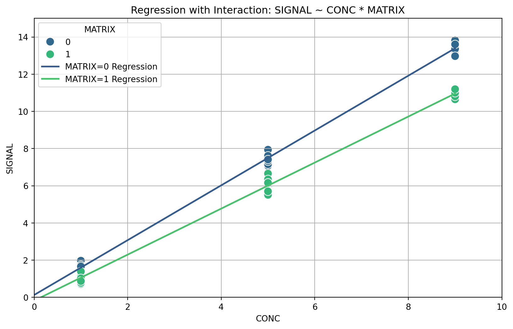
Here both MATRIX p-value < 0.05 and CONC:MATRIX p-value < 0.05, we can exclude the null hypothesis and we can conclude that there is a significant (and negative) effect of the matrix of the intercept and the slope of the response function (Figure 2).

Figure 2: OLS Regression plots

Statistical Considerations

• Ensure sufficient statistical power: at least 10× the number of samples per parameter explored (βₓ).
  
• For exploratory analysis, about 5 replicates per condition (≈30 samples total for 3 concentrations × 2 MATRIXs) is acceptable.
  
• Always verify residual normality, homoscedasticity, and linearity to validate the regression model.